
QuickGraph #5: Australian Open
It’s time for another QuickGraph, this one based on data from the Australian Open tennis tournament. We’re going to use data curated by Jeff Sackmann in the tennis_wta and tennis_atp repositories.

Setting up Neo4j
We’re going to use the following Docker Compose configuration in this blog post:
version: '3.7'

services:
  neo4j:
    image: neo4j:4.0.0-enterprise
    container_name: "quickgraph-aus-open"
    volumes:
      - ./plugins:/plugins
      - ./data:/data
      - ./import:/import
    ports:
      - "7474:7474"
      - "7687:7687"
    environment:
      - "NEO4J_ACCEPT_LICENSE_AGREEMENT=yes"
      - "NEO4J_AUTH=neo4j/neo"
      - NEO4J_apoc_import_file_use__neo4j__config=true
      - NEO4J_apoc_import_file_enabled=true
      - NEO4JLABS_PLUGINS=["apoc"]
We’ll then run the following command to spin up Neo4j:
docker-compose upIf we run that command, we’ll see the following output:
Started quickgraph-aus-open ... done
Attaching to quickgraph-aus-open
quickgraph-aus-open | Changed password for user 'neo4j'.
quickgraph-aus-open | Fetching versions.json for Plugin 'apoc' from https://neo4j-contrib.github.io/neo4j-apoc-procedures/versions.json
quickgraph-aus-open | Installing Plugin 'apoc' from https://github.com/neo4j-contrib/neo4j-apoc-procedures/releases/download/4.0.0.0/apoc-4.0.0.0-all.jar to /plugins/apoc.jar
quickgraph-aus-open | Applying default values for plugin apoc to neo4j.conf
quickgraph-aus-open | Directories in use:
quickgraph-aus-open |   home:         /var/lib/neo4j
quickgraph-aus-open |   config:       /var/lib/neo4j/conf
quickgraph-aus-open |   logs:         /logs
quickgraph-aus-open |   plugins:      /plugins
quickgraph-aus-open |   import:       /import
quickgraph-aus-open |   data:         /var/lib/neo4j/data
quickgraph-aus-open |   certificates: /var/lib/neo4j/certificates
quickgraph-aus-open |   run:          /var/lib/neo4j/run
quickgraph-aus-open | Starting Neo4j.
quickgraph-aus-open | 2020-01-21 22:24:29.976+0000 INFO  ======== Neo4j 4.0.0 ========
quickgraph-aus-open | 2020-01-21 22:24:29.982+0000 INFO  Starting...
quickgraph-aus-open | 2020-01-21 22:24:35.656+0000 INFO  Called db.clearQueryCaches(): Query cache already empty.
quickgraph-aus-open | 2020-01-21 22:24:35.656+0000 INFO  Called db.clearQueryCaches(): Query cache already empty.
quickgraph-aus-open | 2020-01-21 22:24:35.656+0000 INFO  Called db.clearQueryCaches(): Query cache already empty.
quickgraph-aus-open | 2020-01-21 22:24:40.765+0000 INFO  Sending metrics to CSV file at /var/lib/neo4j/metrics
quickgraph-aus-open | 2020-01-21 22:24:40.790+0000 INFO  Bolt enabled on 0.0.0.0:7687.
quickgraph-aus-open | 2020-01-21 22:24:40.791+0000 INFO  Started.
quickgraph-aus-open | 2020-01-21 22:24:40.879+0000 INFO  Server thread metrics have been registered successfully
quickgraph-aus-open | 2020-01-21 22:24:41.723+0000 INFO  Remote interface available at http://0.0.0.0:7474/
Once we see that last line we’re ready to roll.
Exploring the data
Jeff’s repositories includes CSV files containing all the matches on the Women’s WTA tour and Men’s ATP tour.
We won’t be interested in most of the data in these files, but let’s have a look at the 2019 version.
We’ll use the LOAD CSV command to do this:
LOAD CSV WITH HEADERS FROM 'https://raw.githubusercontent.com/JeffSackmann/tennis_wta/master/wta_matches_2019.csv' AS row
RETURN row
LIMIT 1;| row |
|---|
|
We’ve got lots of information to work with here.
We’ll filter the data using the tourney_name so that we only have matches from the Australian Open.
winner_id and loser_id will act as the primary keys for our players and we can combine match_num and tourney_date as the primary key for matches.
winner_name and loser_name give us the human readable version of the players and the score property tells us the result of the match.
Configuring our databases
We’re going to create one database for the men’s matches and one for the women’s matches, with a bit of help from Neo4j 4.0's multi database feature.
:use system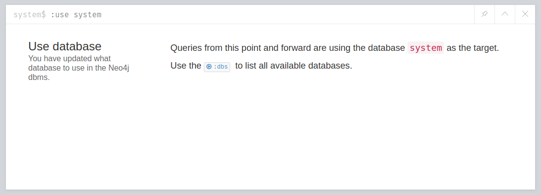
We can then run the following commands to create our databases:
CREATE DATABASE womens;
CREATE DATABASE mens;
Once we’ve done that, let’s return a list of our databases:
SHOW DATABASES;| name | address | role | requestedStatus | currentStatus | error | default |
|---|---|---|---|---|---|---|
"neo4j" |
"0.0.0.0:7687" |
"standalone" |
"online" |
"online" |
"" |
TRUE |
"system" |
"0.0.0.0:7687" |
"standalone" |
"online" |
"online" |
"" |
FALSE |
"womens" |
"0.0.0.0:7687" |
"standalone" |
"online" |
"online" |
"" |
FALSE |
"mens" |
"0.0.0.0:7687" |
"standalone" |
"online" |
"online" |
"" |
FALSE |
Everything’s looking good, we’re ready to start importing the data!
Before we do that let’s change from the system database to the womens database, using the following command:
:use womensImporting the data
We’re going to import the data into the following graph model:
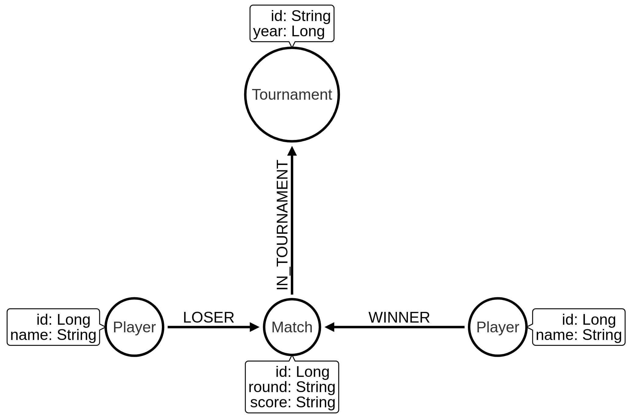
Now let’s set up constraints for our graph. We’re going to create:
-
a unique node property constraint on the
Playerlabel,idproperty andMatchlabel,idproperty. -
a node key constraint on the
Tournamentlabelnameandyearproperties
Those constraints will ensure that we don’t accidentally create duplicate nodes when we import our data. When we create a constraint we also get an index on the label and properties, which will help reduce our import time.
Let’s run the following statements:
CREATE CONSTRAINT ON (p:Player)
ASSERT p.id IS UNIQUE;

CREATE CONSTRAINT ON (m:Match)
ASSERT m.id IS UNIQUE;

CREATE CONSTRAINT ON (t:Tournament)
ASSERT (t.name, t.year) IS NODE KEY;
And now we’ll import the data for the 2019 tournament:
// Only keep Australian open matches
LOAD CSV WITH HEADERS FROM 'https://raw.githubusercontent.com/JeffSackmann/tennis_wta/master/wta_matches_2019.csv' AS row
WITH row, split(row.score, ' ') AS rawSets WHERE row.tourney_name = 'Australian Open'
WITH row, row.tourney_date + '_' + row.match_num AS matchId

// Create nodes for Tournaments, Matches, and Players
MERGE (t:Tournament {name: row.tourney_name, year: date(row.tourney_date).year})

MERGE (m:Match {id: matchId})
SET m.round = row.round, m.score = row.score

MERGE (p1:Player {id: row.winner_id})
SET p1.name = row.winner_name

MERGE (p2:Player {id: row.loser_id})
SET p2.name = row.loser_name

// Create relationships between nodes
MERGE (p1)-[:WINNER]->(m)
MERGE (p2)-[:LOSER]->(m)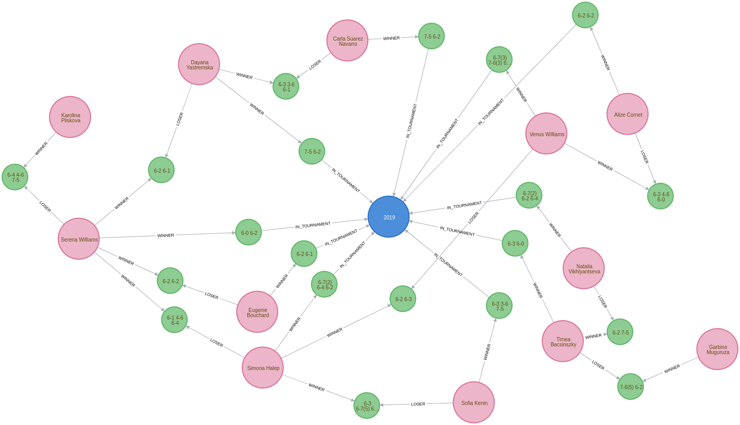
MERGE (m)-[:IN_TOURNAMENT]->(t)0 rows available after 1218 ms, consumed after another 0 ms Added 256 nodes, Created 381 relationships, Set 765 properties, Added 256 labels |
We can see a sample of the imported graph in the Neo4j Browser visualisation below:
Let’s now load in the data for some of the other years. Jeff Sackmann has curated data going back to 1968, but we’ll only load data from the year 2000 onwards.
We could import all the tournaments in one transaction, but our import will be much quicker if we use the apoc.periodic.iterate procedure from APOC, Neo4j’s standard library.
CALL apoc.periodic.iterate(
  "UNWIND range(2000, 2019) AS year RETURN year",
  "WITH 'https://raw.githubusercontent.com/JeffSackmann/tennis_wta/master/wta_matches_' AS base,
        year
   LOAD CSV WITH HEADERS FROM base + year + '.csv' AS row
   WITH row, split(row.score, ' ') AS rawSets WHERE row.tourney_name = 'Australian Open'
   WITH row, row.tourney_date + '_' + row.match_num AS matchId

   MERGE (t:Tournament {name: row.tourney_name, year: date(row.tourney_date).year})

   MERGE (m:Match {id: matchId})
   SET m.round = row.round, m.score = row.score

   MERGE (p1:Player {id: row.winner_id})
   SET p1.name = row.winner_name

   MERGE (p2:Player {id: row.loser_id})
   SET p2.name = row.loser_name

   MERGE (p1)-[:WINNER]->(m)
   MERGE (p2)-[:LOSER]->(m)
   MERGE (m)-[:IN_TOURNAMENT]->(t)
", {})| batches | total | timeTaken | committedOperations | failedOperations | failedBatches | retries | errorMessages | batch | operations | wasTerminated | failedParams |
|---|---|---|---|---|---|---|---|---|---|---|---|
1 |
20 |
13 |
20 |
0 |
0 |
0 |
{} |
{total: 1, committed: 1, failed: 0, errors: {}} |
{total: 20, committed: 20, failed: 0, errors: {}} |
FALSE |
{} |
One interesting thing about this dataset is that it has implicit relationships between tournaments and between matches.
For example, the 2019 tournament is the NEXT_TOURNAMENT after the 2018 tournament and if a player wins their 1st round match, there could be a NEXT_MATCH relationship to their 2nd round match.
I think having these explicit relationships will enable some cool path based queries.
We’ll need to write a query that collects these nodes in order and uses the apoc.nodes.link procedure to create the new relationships.
The following Cypher statements create the relationships:
// Store the rounds in a list that will be used to sort matches
:params rounds: ["R128", "R64", "R32", "R16", "QF", "SF", "F"];

// Build a map from that list
WITH apoc.map.fromLists( $rounds, range(0, size($rounds)-1)) AS rounds

// Collect matches grouped by player and tournament, ordered by round
MATCH (t:Tournament)<-[:IN_TOURNAMENT]-(m:Match)<--(player)
WITH player, m, t
ORDER BY player, rounds[m.round]
WITH player, t, collect(m) AS matches
WHERE size(matches) > 1

// Add NEXT_MATCH relationship between adjacent matches
CALL apoc.nodes.link(matches, "NEXT_MATCH")
RETURN count(*);

// Collect tournaments ordered by year
MATCH (t:Tournament)
WITH t
ORDER BY t.year
WITH collect(t) AS tournaments

// Add NEXT_TOURNAMENT between adjacent matches
CALL apoc.nodes.link(tournaments, "NEXT_TOURNAMENT")
RETURN count(*);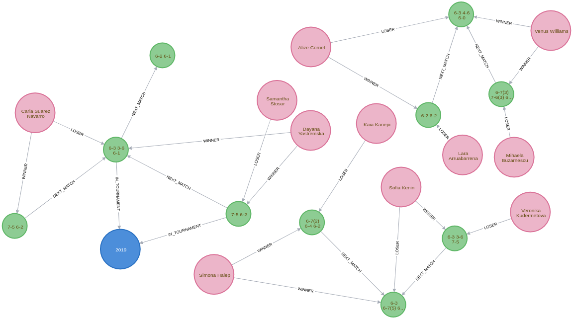
The full import script for the women’s tournament is available in the import_womens.cypher file. And there is an equivalent import script for the men’s tournament in the import_mens.cypher file.
Querying the graph
Alright, it’s time to start writing some queries!
Who won each of the tournaments?
Let’s start with a simple query to find out the finalists in each tournament and the result of the final match:
MATCH (winner:Player)-[:WINNER]->(match:Match {round: "F"})<-[:LOSER]-(loser),
      (match)-[:IN_TOURNAMENT]->(tournament)
RETURN tournament.year AS year, winner.name AS winner,
       loser.name AS loser, match.score AS score
ORDER BY tournament.year| year | winner | loser | score |
|---|---|---|---|
2000 |
"Lindsay Davenport" |
"Martina Hingis" |
"6-1 7-5" |
2001 |
"Jennifer Capriati" |
"Martina Hingis" |
"6-4 6-3" |
2002 |
"Jennifer Capriati" |
"Martina Hingis" |
"4-6 7-6(7) 6-2" |
2003 |
"Serena Williams" |
"Venus Williams" |
"7-6(4) 3-6 6-4" |
2004 |
"Justine Henin" |
"Kim Clijsters" |
"6-3 4-6 6-3" |
2005 |
"Serena Williams" |
"Lindsay Davenport" |
"2-6 6-3 6-0" |
2006 |
"Amelie Mauresmo" |
"Justine Henin" |
"6-1 2-0 RET" |
2007 |
"Serena Williams" |
"Maria Sharapova" |
"6-1 6-2" |
2008 |
"Maria Sharapova" |
"Ana Ivanovic" |
"7-5 6-3" |
2009 |
"Serena Williams" |
"Dinara Safina" |
"6-0 6-3" |
2010 |
"Serena Williams" |
"Justine Henin" |
"6-4 3-6 6-2" |
2011 |
"Kim Clijsters" |
"Na Li" |
"3-6 6-3 6-3" |
2012 |
"Victoria Azarenka" |
"Maria Sharapova" |
"6-3 6-0" |
2013 |
"Victoria Azarenka" |
"Na Li" |
"4-6 6-4 6-3" |
2014 |
"Na Li" |
"Dominika Cibulkova" |
"7-6(3) 6-0" |
2015 |
"Serena Williams" |
"Maria Sharapova" |
"6-3 7-6(5)" |
2016 |
"Angelique Kerber" |
"Serena Williams" |
"6-4 3-6 6-4" |
2017 |
"Serena Williams" |
"Venus Williams" |
"6-4 6-4" |
2018 |
"Caroline Wozniacki" |
"Simona Halep" |
"7-6(2) 3-6 6-4" |
2019 |
"Naomi Osaka" |
"Petra Kvitova" |
"7-6(2) 5-7 6-4" |
We’ve got lots of different winners here and a few players who have won the tournament multiple times. Serena Williams has won the tournament an incredible 7 times in 20 years!
What was Osaka’s route to the 2019 final?
The final is the most important match, but what route did the winner take to get there? Let’s have a look at Naomi Osaka’s journey to the 2019 final:
// Find all the matches that the winner of the tournament played
MATCH path = (p:Player)-[:WINNER]->(match:Match {round: "F"})<-[:NEXT_MATCH*]-(m)<-[:WINNER]-(p)

// Only get the winner of the 2019 tournament
// Only get the longest path of NEXT_MATCH relationships that includes all matches
// played by the winner
WHERE not((m)<-[:NEXT_MATCH]-()) AND (match)-[:IN_TOURNAMENT]-(:Tournament {year: 2019})

// Find the winners and losers of all the matches in which the winner participated
RETURN path,
       [node in nodes(path) WHERE node:Match | [p = (p1)-[:WINNER]->(node)<-[:LOSER]-(p2) | p]];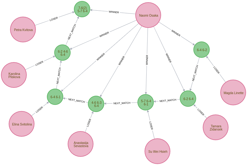
Who lost the final, but won it the next year?
In this query we’re going to try and find players that lost the final, but then won the tournament the following year:
MATCH (player)-[:LOSER]->(:Match {round: "F"})-[:IN_TOURNAMENT]->(t)-[:NEXT_TOURNAMENT]->(t2),
      (player)-[:WINNER]->(:Match {round: "F"})-[:IN_TOURNAMENT]->(t2)
RETURN player.name AS player, t.year, t2.year| player | t.year | t2.year |
|---|---|---|
"Maria Sharapova" |
2007 |
2008 |
"Na Li" |
2013 |
2014 |
"Serena Williams" |
2016 |
2017 |
Just the three players fixed their heart break at losing the final as quickly as possible.
Who lost the final, but subsequently won the tournament?
Are there any players who lost the final but won it at some future tournament even if it wasn’t the next year?
To do that we’ll add a * to the NEXT_TOURNAMENT part of the query, which will cause the Cypher engine to look at all future tournaments rather than just the following year:
MATCH (player)-[:LOSER]->(:Match {round: "F"})-[:IN_TOURNAMENT]->(t)-[:NEXT_TOURNAMENT*]->(t2),
      (player)-[:WINNER]->(:Match {round: "F"})-[:IN_TOURNAMENT]->(t2)
RETURN player.name, t.year, t2.year| player | t.year | t2.year |
|---|---|---|
"Maria Sharapova" |
2007 |
2008 |
"Kim Clijsters" |
2004 |
2011 |
"Na Li" |
2013 |
2014 |
"Na Li" |
2011 |
2014 |
"Serena Williams" |
2016 |
2017 |
We get the 3 players from the previous query as well as Kim Clijsters and Li Na. Li Na actually lost the final twice before winning it in 2014.
How long did players wait from their first final defeat until their first win?
We could tweak this query slightly to find the number of years that passed between a player losing their first final and winning their first final. We’ll also add an additional filter so that we exclude players who have already won the tournament before they lost in the final.
// Find the first year that a player lost the final
MATCH (player)-[:LOSER]->(:Match {round: "F"})-[:IN_TOURNAMENT]->(t)

// Where they haven't previously won the tournament
WHERE not((player)-[:WINNER]->(:Match {round: "F"})-[:IN_TOURNAMENT]->()-[:NEXT_TOURNAMENT*]->(t))

WITH player, t
ORDER BY player, t.year
WITH player, collect(t)[0] AS firstLoss

// Find the first year that a player won the final after that loss
MATCH (firstLoss)-[:NEXT_TOURNAMENT*]->(t2),
      (player)-[:WINNER]->(:Match {round: "F"})-[:IN_TOURNAMENT]->(t2)
      WITH player, firstLoss, t2
ORDER BY player, t2.year
WITH player, firstLoss, collect(t2)[0] AS firstWin

RETURN player.name, firstLoss.year, firstWin.year, firstWin.year - firstLoss.year AS theWait
ORDER BY theWait DESC| player.name | firstLoss.year | firstWin.year | theWait |
|---|---|---|---|
"Kim Clijsters" |
2004 |
2011 |
7 |
"Na Li" |
2011 |
2014 |
3 |
"Maria Sharapova" |
2007 |
2008 |
1 |
Clijsters had to wait the longest and Serena had in fact previously won the tournament, so she isn’t returned in the results anymore.
We can run this query against the Men’s database as well by switching to that database using the command :use mens and re-running the query.
| player.name | firstLoss.year | firstWin.year | theWait |
|---|---|---|---|
"Marat Safin" |
2002 |
2005 |
3 |
Marat Safin is the only one, and he didn’t have to wait too long to win the tournament.
What about sets?
Tennis commentators often talk about the number of sets that the winner of the tournament lost along the way, so that’s what we’re going to explore next.
At the moment the sets won is hidden inside the score property on the Match nodes.
We’re going to create one node per set played and connect those sets to the existing graph, as shown in the diagram below:
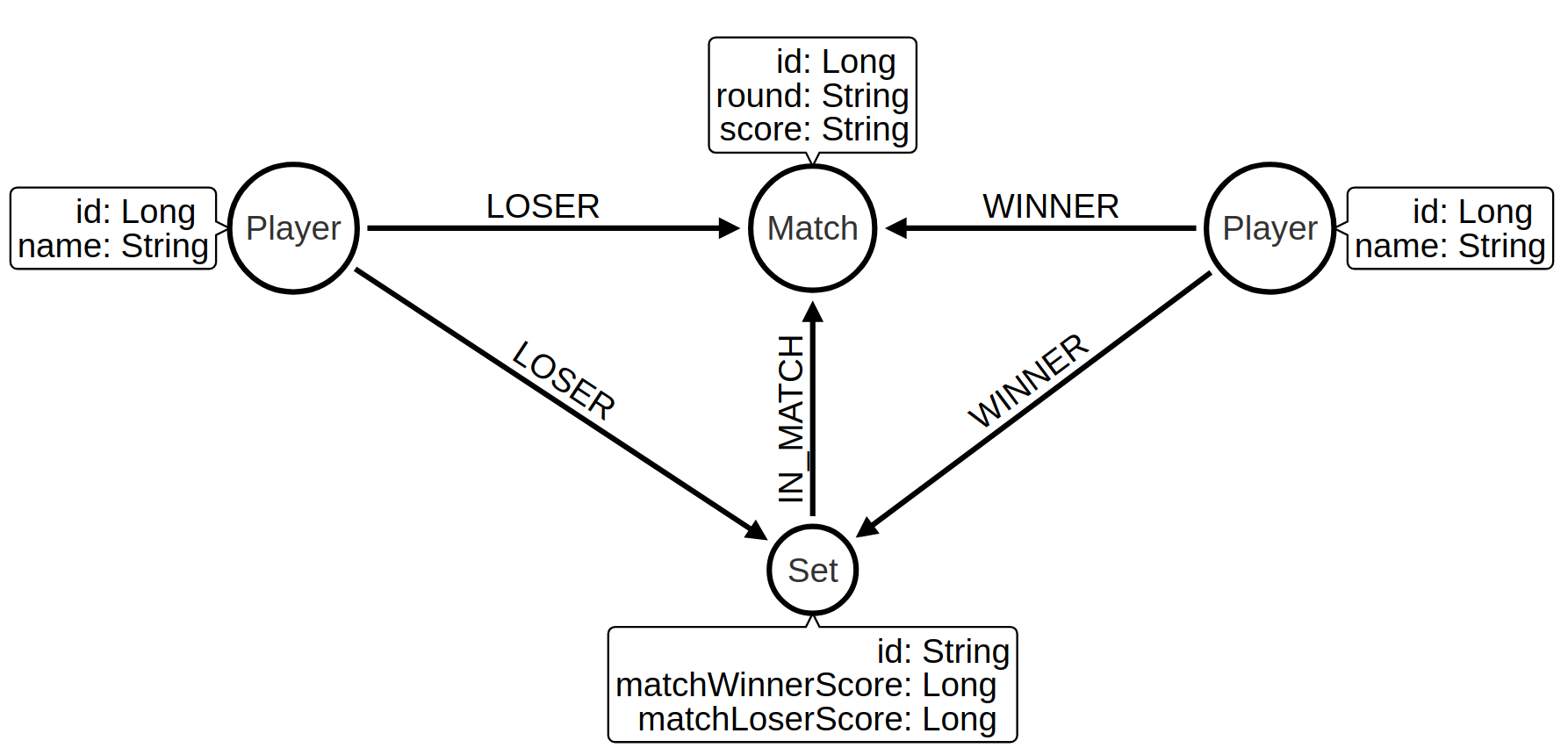
We can update the graph with the following Cypher statement:
CALL apoc.periodic.iterate(
"UNWIND range(2000, 2019) AS year RETURN year",
"WITH 'https://raw.githubusercontent.com/JeffSackmann/tennis_wta/master/wta_matches_' AS base,
year
LOAD CSV WITH HEADERS FROM base + year + '.csv' AS row
WITH row, split(row.score, ' ') AS rawSets WHERE row.tourney_name = 'Australian Open'
WITH row, rawSets,
[set in rawSets |
apoc.text.regexGroups(set, \"(\\\\d{1,2})-(\\\\d{1,2})\")[0][1..]] AS sets,
row.tourney_date + '_' + row.match_num AS matchId
MATCH (m:Match {id: matchId})
MATCH (p1:Player {id: row.winner_id})
MATCH (p2:Player {id: row.loser_id})
WITH m, sets, rawSets, matchId, p1, p2
UNWIND range(0, size(sets)-1) AS setNumber
MERGE (s:Set {id: matchId + '_' + setNumber})
SET s.matchWinnerScore = toInteger(sets[setNumber][0]),
s.matchLoserScore = toInteger(sets[setNumber][1]),
s.score = rawSets[setNumber],
s.number = setNumber +1
MERGE (s)-[:IN_MATCH]->(m)
FOREACH(ignoreMe IN CASE WHEN s.matchWinnerScore >= s.matchLoserScore THEN [1] ELSE [] END |
MERGE (p1)-[:WINNER]->(s)
MERGE (p2)-[:LOSER]->(s))
FOREACH(ignoreMe IN CASE WHEN s.matchWinnerScore < s.matchLoserScore THEN [1] ELSE [] END |
MERGE (p1)-[:LOSER]->(s)
MERGE (p2)-[:WINNER]->(s))
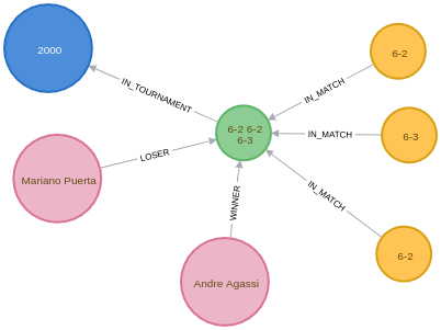
", {});We can see a sample of the graph with sets included in the Neo4j Browser visualisation below:
Now let’s write some queries against the updated model.
Querying the graph: Sets Edition
Did anyone win the tournament without losing a set?
Let’s start by finding out if any players had a perfect tournament i.e. they won it without losing a set. The following query reveals all:
MATCH (winner:Player)-[:WINNER]->(:Match {round: "F"})-[:IN_TOURNAMENT]->(t)
MATCH (winner)-[:WINNER]->(match)-[:IN_TOURNAMENT]->(t)
WITH winner, match, t
ORDER BY t.year
WITH winner, t,
     collect([(match)<-[:IN_MATCH]-(set:Set)
              WHERE (winner)-[:LOSER]->(set) | set
             ][0]) AS setDropped
WHERE size(setDropped) = 0
RETURN winner.name AS winner, t.year AS year| winner | year |
|---|---|
"Roger Federer" |
2007 |
Just the one on the men’s side. What about the women’s?
| winner | year |
|---|---|
"Lindsay Davenport" |
2000 |
"Maria Sharapova" |
2008 |
"Serena Williams" |
2017 |
Only three players here. So that means in most tournaments the winner loses a set somewhere along the way.
Did the winner drop any sets?
Let’s tweak that previous query a bit to return the number of matches in which the winner lost a set and the total number of sets lost:
WITH apoc.map.fromLists( $rounds, range(0, size($rounds)-1)) AS rounds
MATCH (winner:Player)-[:WINNER]->(:Match {round: "F"})-[:IN_TOURNAMENT]->(t)
MATCH (winner)-[:WINNER]->(match)-[:IN_TOURNAMENT]->(t),
      (match)<-[:LOSER]-(opponent)
WHERE (winner)-[:LOSER]->(:Set)-[:IN_MATCH]->(match)

WITH *
ORDER BY rounds[match.round]

WITH winner, t,
     collect({round: match.round, opponent: opponent.name, score: match.score }) AS matches,
     collect([(match)<-[:IN_MATCH]-(set)<-[:LOSER]-(winner) | set]) AS sets
RETURN winner.name AS winner, t.year AS year, size(matches) AS count,
       size(apoc.coll.flatten(sets)) AS sets,  matches
ORDER BY count DESC
LIMIT 5| winner | year | count | sets | matches |
|---|---|---|---|---|
"Thomas Johansson" |
2002 |
6 |
7 |
[{score: "6-1 3-6 7-6(2) 6-4", round: "R128", opponent: "Jacobo Diaz"}, {score: "5-7 6-2 6-2 6-4", round: "R32", opponent: "Younes El Aynaoui"}, {score: "6-7(8) 6-2 6-0 6-4", round: "R16", opponent: "Adrian Voinea"}, {score: "6-0 2-6 6-3 6-4", round: "QF", opponent: "Jonas Bjorkman"}, {score: "7-6(5) 0-6 4-6 6-3 6-4", round: "SF", opponent: "Jiri Novak"}, {score: "3-6 6-4 6-4 7-6(4)", round: "F", opponent: "Marat Safin"}] |
"Roger Federer" |
2017 |
4 |
7 |
[{score: "7-5 3-6 6-2 6-2", round: "R128", opponent: "Jurgen Melzer"}, {score: "6-7(4) 6-4 6-1 4-6 6-3", round: "R16", opponent: "Kei Nishikori"}, {score: "7-5 6-3 1-6 4-6 6-3", round: "SF", opponent: "Stanislas Wawrinka"}, {score: "6-4 3-6 6-1 3-6 6-3", round: "F", opponent: "Rafael Nadal"}] |
"Marat Safin" |
2005 |
4 |
5 |
[{score: "6-4 3-6 6-3 6-4", round: "R32", opponent: "Mario Ancic"}, {score: "4-6 7-6(1) 7-6(5) 7-6(2)", round: "R16", opponent: "Olivier Rochus"}, {score: "5-7 6-4 5-7 7-6(6) 9-7", round: "SF", opponent: "Roger Federer"}, {score: "1-6 6-3 6-4 6-4", round: "F", opponent: "Lleyton Hewitt"}] |
"Roger Federer" |
2006 |
4 |
5 |
[{score: "6-4 6-0 3-6 4-6 6-2", round: "R16", opponent: "Tommy Haas"}, {score: "6-4 3-6 7-6(7) 7-6(5)", round: "QF", opponent: "Nikolay Davydenko"}, {score: "6-3 5-7 6-0 6-2", round: "SF", opponent: "Nicolas Kiefer"}, {score: "5-7 7-5 6-0 6-2", round: "F", opponent: "Marcos Baghdatis"}] |
"Stanislas Wawrinka" |
2014 |
4 |
5 |
[{score: "6-3 6-3 6-7(4) 6-4", round: "R64", opponent: "Alejandro Falla"}, {score: "2-6 6-4 6-2 3-6 9-7", round: "QF", opponent: "Novak Djokovic"}, {score: "6-3 6-7(1) 7-6(3) 7-6(4)", round: "SF", opponent: "Tomas Berdych"}, {score: "6-3 6-2 3-6 6-3", round: "F", opponent: "Rafael Nadal"}] |
So Thomas Johansson had the toughest route to the title, dropping a set in every match except for the 2nd round (R64).
We could probably think of some other set based queries to execute against this dataset, but this blog post has already got much longer than I expected so I think we’ll leave it there for now.
What’s interesting about this QuickGraph?
I’ve always wanted to put tennis matches into a graph, but I was always struggling to think what type of graphy queries could be run against such a dataset. And for most of this blog post I wasn’t really convinced that a graph was allowing us to write very interesting queries.
Things got more interesting in the last section where we did set analysis. I found having the data in a graph structure made was helpful for answering these questions, especially when we were looking for the non existence of a relationship. I do still wonder if there’s a cleaner way to write those queries.
Thanks against to Jeff Sackmann for curating the datasets. You saved me a lot of work preparing the data!
About the author
I'm currently working on short form content at ClickHouse. I publish short 5 minute videos showing how to solve data problems on YouTube @LearnDataWithMark. I previously worked on graph analytics at Neo4j, where I also co-authored the O'Reilly Graph Algorithms Book with Amy Hodler.