22 Dec 2019

QuickGraph #2: Guardian Top 100 Male Footballers

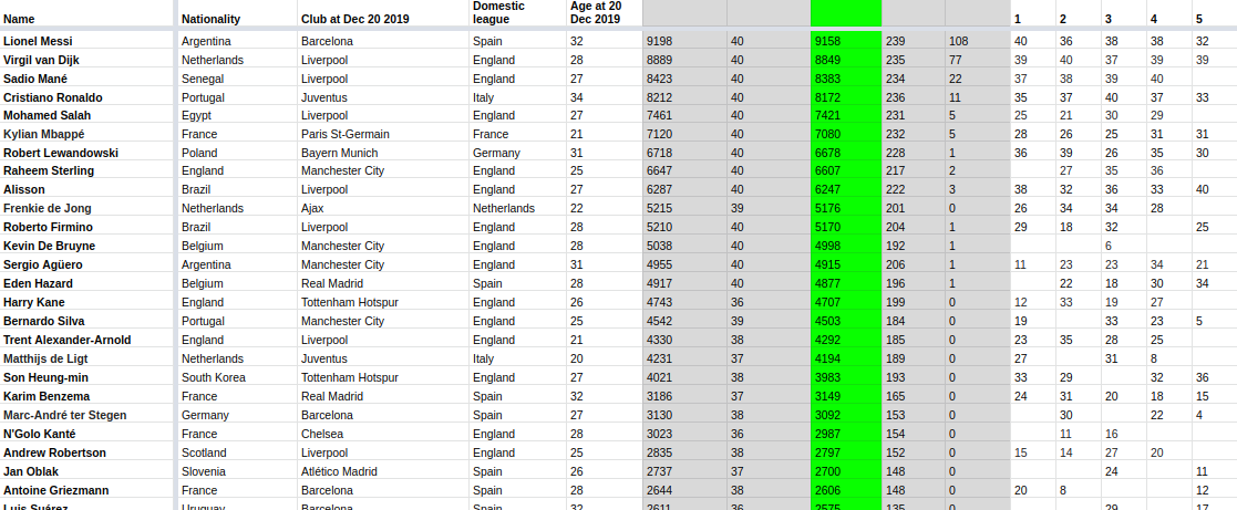
Over the last week the Guardian have been counting down their top 100 male footballers of 2019, and on Friday they also published a Google sheet containing all the votes, which seemed like a perfect candidate for a QuickGraph.

We can see a preview of the Google sheet in the printscreen below:

We can also download Google Sheets in CSV format based on the following URI template:

https://docs.google.com/spreadsheets/d/KEY/export?format=csv&id=KEY&gid=SHEET_ID

where:

KEY is the spreadsheet id, in our case 1f4nc8vehOiZhEB2_3L2bvXTpag29VcEKJ0PJeo5Runc
SHEET_ID is the sheet, in our case 3

Exploring the data

We can use Neo4j’s LOAD CSV tool to explore the data. The following query returns the 1st player on the list:

WITH "1f4nc8vehOiZhEB2_3L2bvXTpag29VcEKJ0PJeo5Runc" AS id
WITH "https://docs.google.com/spreadsheets/d/" + id + "/export?format=csv&id=" + id + "&gid=3" AS uri
LOAD CSV FROM uri AS row
WITH row SKIP 4 LIMIT 1
RETURN row

If we run that query, we’ll see the following output:

Table 1. Results
row
["1", "2", "3", "1", "2", "1", "2", "1", "Lionel Messi", "Argentina", "Barcelona", "Spain", "32", "31", "9198", "40", "9158", "239", "108", "40", "36", "38", "38", "32", "40", "13", "39", "40", "40", "39", "30", "40", "40", "39", "37", "40", "38", "39", "39", "40", "39", "38", "38", "40", "38", "40", "40", "40", "39", "39", "38", "38", "39", "40", "40", "40", "40", "38", "40", "40", "40", "39", "40", "40", "39", "40", "39", "37", "39", "40", "40", "39", "40", "39", "37", "36", "40", "39", "38", "40", "39", "39", "40", "40", "34", "40", "40", "40", "40", "39", "38", "40", "40", "39", "40", "38", "40", "40", "39", "39", "35", "40", "40", "39", "39", "39", "38", "40", "39", "39", "36", "39", "40", "24", "40", "39", "30", "39", "39", "40", "40", "39", "39", "39", "37", "40", "35", "40", "35", "39", "39", "39", "37", "40", "39", "40", "38", "40", "40", "39", "40", "39", "39", "40", "37", "40", "36", "39", "40", "39", "38", "39", "40", "40", "40", "38", "22", "38", "39", "40", "39", "37", "40", "40", "40", "40", "40", "38", "40", "38", "40", "39", "40", "40", "39", "40", "40", "22", "39", "40", "40", "40", "40", "38", "39", "39", "38", "39", "39", "19", "40", "32", "40", "40", "40", "30", "39", "40", "40", "40", "38", "40", "40", "40", "39", "40", "40", "37", "40", "36", "37", "38", "39", "40", "39", "40", "40", "40", "38", "39", "40", "40", "40", "38", "39", "36", "39", "30", "38", "40", "40", "39", "39", "40", "39", "40", "40", "37", "40", "40", "39", "40", "39", "38", "40", "38", "39", "39", "38", "38", "40", "40", "39", "40", "40", "39", "38", "40"]

We’re not interested in the first 8 columns, but we do want to capture the next 4 columns, which contain the player’s name, nationality, club, and the country where that club competes. We’ll then skip the next 7 columns until we get to the votes given by each of the judges.

Importing the data

We’re going to import the data into the following graph model:

Before we run any import statements, we’ll make sure we don’t accidentally import any duplicates by creating unique constraints on each of the node labels:

CALL apoc.schema.assert(null,{Judge:['id'], Player:["name"], Country:["name"], Club:["name"]});

We can run the following query to check that they’ve been created:

Table 2. Results
description	indexName	tokenNames	properties	state	type	progress	provider	id	failureMessage
"INDEX ON :Club(name)"	"index_7"	["Club"]	["name"]	"ONLINE"	"node_unique_property"	100.0	{version: "1.0", key: "native-btree"}	7	""
"INDEX ON :Country(name)"	"index_1"	["Country"]	["name"]	"ONLINE"	"node_unique_property"	100.0	{version: "1.0", key: "native-btree"}	1	""
"INDEX ON :Judge(id)"	"index_10"	["Judge"]	["id"]	"ONLINE"	"node_unique_property"	100.0	{version: "1.0", key: "native-btree"}	10	""
"INDEX ON :Player(name)"	"index_4"	["Player"]	["name"]	"ONLINE"	"node_unique_property"	100.0	{version: "1.0", key: "native-btree"}	4	""

All good so far. Now let’s import the votes.

We’re going to use the same LOAD CSV tool that we used to explore the data. Importing the data is a bit fiddly because rows 105 and 186 don’t contain players, so we need to skip those rows.

The following LOAD CSV statement imports the top 100 players, along with their club, country, and votes:

WITH "1f4nc8vehOiZhEB2_3L2bvXTpag29VcEKJ0PJeo5Runc" AS id
WITH "https://docs.google.com/spreadsheets/d/" + id + "/export?format=csv&id=" + id + "&gid=3" AS uri
LOAD CSV FROM uri AS row
WITH row SKIP 4 LIMIT 100
MERGE (player:Player {name: row[8]})
SET player.rawScore = toInteger(row[14]), player.score = toInteger(row[16])
MERGE (country:Country {name: row[9]})
MERGE (club:Club {name: row[10]})
MERGE (clubCountry:Country {name: row[11]})
MERGE (player)-[:NATIONALITY]->(country)
MERGE (player)-[:PLAYS_FOR]->(club)
MERGE (club)-[:PLAY_IN]->(clubCountry)

FOREACH(index in range(19, size(row)-1) |
  MERGE (judge:Judge {id: index-18})
  FOREACH(ignoreMe IN CASE WHEN row[index] is null THEN [] ELSE [1] END |
	MERGE (judge)-[voted:VOTED]->(player)
	SET voted.score = toInteger(row[index])
));

To import the rest of the players we’ll have to vary the SKIP and LIMIT values on the 4th line of the query The GitHub gist below includes statements that import the votes for all players:

We can see a sample of the imported graph in the Neo4j Browser visualisation below:

Querying the graph

Now that we’ve imported the data, it’s time to start querying it. The Google sheet already contains the answers to the following questions:

How many judges included each player in their top 40?
How many judges voted for a player as their number 1?
What’s the top ranking that a player received?

Let’s see what else we can learn. The queries that follow use Neo4j’s Cypher query language.

How many judges included the top 5 in their top 5?

MATCH (player:Player)
WHERE exists(player.score)
WITH player ORDER BY player.score DESC LIMIT 5
MATCH (player)<-[voted:VOTED]-()
WHERE voted.score >= 36
WITH player, 41-voted.score AS rank, count(*) AS count
RETURN player.name AS player,
       apoc.map.fromPairs(collect([rank, count])) AS votes,
       player.score AS score;

Table 3. How many judges included the top 5 in their top 5?
player	votes	score
"Lionel Messi"	{`1`: 108, `2`: 69, `3`: 31, `4`: 10, `5`: 6}	9158
"Virgil van Dijk"	{`1`: 77, `2`: 59, `3`: 30, `4`: 30, `5`: 8}	8849
"Sadio Mané"	{`1`: 22, `2`: 34, `3`: 46, `4`: 36, `5`: 28}	8383
"Cristiano Ronaldo"	{`1`: 11, `2`: 29, `3`: 53, `4`: 31, `5`: 28}	8172
"Mohamed Salah"	{`1`: 5, `2`: 8, `3`: 16, `4`: 24, `5`: 29}	7421

We can see that the judges overwhelmingly have Messi and van Dijk in their top 2. This is not that surprising given that they finished 1st and 2nd in the The Best FIFA Football Awards 2019 and 2019 Ballon d’Or.

Did any judges get the top 3 exactly right?

Which judges got the top 3 exactly correct?

MATCH (player1:Player {name: "Lionel Messi"})<-[:VOTED {score: 40}]-(judge)
MATCH (player2:Player {name: "Virgil van Dijk"})<-[:VOTED {score: 39}]-(judge)
MATCH (player3:Player {name: "Sadio Mané"})<-[:VOTED {score: 38}]-(judge)
WITH collect(judge.id) AS judges
RETURN size(judges) AS count, judges

Table 4. Which judges got the top 3 exactly correct?
count	judges
14	[179, 145, 102, 239, 187, 204, 220, 215, 144, 51, 202, 42, 79, 218]

Only 14 out of 239 (or 6% of the) judges got the top 3 exactly right. Football is clearly a game of different opinions!

Next let’s see which clubs have fared best.

Which club has the most players on the list?

MATCH (club:Club)<-[:PLAYS_FOR]-(:Player)
RETURN club.name AS club, count(*) AS count
ORDER BY count DESC
LIMIT 10

Table 5. Which club has the most players on the list?
club	count
"Real Madrid"	19
"Manchester City"	17
"Liverpool"	15
"Juventus"	14
"Bayern Munich"	14
"Barcelona"	14
"Paris St-Germain"	12
"Chelsea"	11
"Atlético Madrid"	10
"Tottenham Hotspur"	9

Manchester City and Liverpool had very strong years, so it’s not surprising to see that they have a lot of players on the list. Real Madrid having the most players is a strange one given their relatively poor year.

Perhaps the players that they have on the list didn’t receive many votes. Let’s tweak the query to sum the voting scores given to the players that play for those clubs

Which clubs have the highest ranking players on the list?

MATCH (club:Club)<-[:PLAYS_FOR]-(player:Player)
OPTIONAL MATCH (player)<-[voted:VOTED]-()
RETURN club.name, count(DISTINCT player) AS count, sum(voted.score) AS totalScore
ORDER BY totalScore DESC
LIMIT 10

Table 6. Which clubs have the highest ranking players on the list?
club	count	totalScore
"Liverpool"	15	46803
"Manchester City"	17	25915
"Barcelona"	14	19154
"Juventus"	14	15265
"Real Madrid"	19	13078
"Paris St-Germain"	12	12500
"Ajax"	9	11608
"Tottenham Hotspur"	9	10956
"Bayern Munich"	14	10255
"Atlético Madrid"	10	4950

That’s more like it.

Liverpool are way clear at the top, which makes sense given they won the Champions League and have a big lead in this year’s Premier League season. After them come the 2018/2019 winners of the Premier League, La Liga, and Serie A, before we find Real Madrid in 5th place.

The top 10 contains 3 clubs that play in England, 3 clubs that play in Spain, and 1 each from the Netherlands, Germany, France, and Italy. Let’s next see which countries have the highest ranking players on the whole list.

Which countries have the highest ranking players on the list?

MATCH (club:Club)<-[:PLAYS_FOR]-(player:Player)
OPTIONAL MATCH (player)<-[voted:VOTED]-()
WITH club, count(DISTINCT player) AS count, sum(voted.score) AS totalScore
ORDER BY club, totalScore DESC
MATCH (club)-[:PLAY_IN]->(country)
RETURN country.name, sum(count) AS count, sum(totalScore) AS totalScore,
       collect([club.name, totalScore])[..5] AS clubs
ORDER BY totalScore DESC
LIMIT 5

Table 7. Which clubs have the highest ranking players on the list?
club	count	totalScore	clubs
"England"	85	94221	[["Liverpool", 46803], ["Manchester City", 25915], ["Tottenham Hotspur", 10956], ["Chelsea", 4273], ["Arsenal", 2635]]
"Spain"	62	37926	[["Barcelona", 19154], ["Real Madrid", 13078], ["Atlético Madrid", 4950], ["Villarreal", 206], ["Valencia", 210]]
"Italy"	49	21167	[["Juventus", 15269], ["Napoli", 2638], ["Internazionale", 1174], ["Lazio", 491], ["Atalanta", 504]]
"Germany"	33	13882	[["Bayern Munich", 10255], ["Borussia Dortmund", 2655], ["RB Leipzig", 576], ["Bayer Leverkusen", 279], ["Borussia Mönchengladbach", 72]]
"France"	26	13170	[["Paris St-Germain", 12500], ["Lyon", 368], ["Lille", 108], ["Monaco", 52], ["Nice", 71]]

Although both England and Spain had 3 players each in the top 10, the total score of those playing in England is almost twice as high as for those in Spain. This is mostly due to the high ranking of Manchester City and Liverpool players. Looking at the rest of the list, we can see that the top 5 countries are the big 5 European leagues, which is also where the majority of football’s money lives.

That’s all I can think of for now, but if you can think of any other analysis we can do on this data, let me know in the comments!

About the author

I'm currently working on short form content at ClickHouse. I publish short 5 minute videos showing how to solve data problems on YouTube @LearnDataWithMark. I previously worked on graph analytics at Neo4j, where I also co-authored the O'Reilly Graph Algorithms Book with Amy Hodler.