19 May 2018

Interpreting Word2vec or GloVe embeddings using scikit-learn and Neo4j graph algorithms

A couple of weeks I came across a paper titled Parameter Free Hierarchical Graph-Based Clustering for Analyzing Continuous Word Embeddings via Abigail See's blog post about ACL 2017.

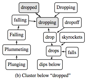
The paper explains an algorithm that helps to make sense of word embeddings generated by algorithms such as Word2vec and GloVe.

I’m fascinated by how graphs can be used to interpret seemingly black box data, so I was immediately intrigued and wanted to try and reproduce their findings using Neo4j.

This is my understanding of the algorithm:

Create a nearest neighbour graph (NNG) of our embedding vectors, where each vector can only have one relationship to its nearest neighbour
Run the connected components algorithm over that NNG to derive clusters of words
For each cluster define a macro vertex - this could be the most central word in the cluster or the most popular word
Create a NNG of the macro vertices
Repeat steps 2 and 3 until we have only one cluster left

We can use the Neo4j graph algorithms library for Step 2 and I initially tried to brute force Step 1 before deciding to use scikit-learn for this part of the algorithm.

$ head -n1 data/small_glove.txt
the -0.038194 -0.24487 0.72812 -0.39961 0.083172 0.043953 -0.39141 0.3344 -0.57545 0.087459 0.28787 -0.06731 0.30906 -0.26384 -0.13231 -0.20757 0.33395 -0.33848 -0.31743 -0.48336 0.1464 -0.37304 0.34577 0.052041 0.44946 -0.46971 0.02628 -0.54155 -0.15518 -0.14107 -0.039722 0.28277 0.14393 0.23464 -0.31021 0.086173 0.20397 0.52624 0.17164 -0.082378 -0.71787 -0.41531 0.20335 -0.12763 0.41367 0.55187 0.57908 -0.33477 -0.36559 -0.54857 -0.062892 0.26584 0.30205 0.99775 -0.80481 -3.0243 0.01254 -0.36942 2.2167 0.72201 -0.24978 0.92136 0.034514 0.46745 1.1079 -0.19358 -0.074575 0.23353 -0.052062 -0.22044 0.057162 -0.15806 -0.30798 -0.41625 0.37972 0.15006 -0.53212 -0.2055 -1.2526 0.071624 0.70565 0.49744 -0.42063 0.26148 -1.538 -0.30223 -0.073438 -0.28312 0.37104 -0.25217 0.016215 -0.017099 -0.38984 0.87424 -0.72569 -0.51058 -0.52028 -0.1459 0.8278 0.27062

Imports

First let’s load in the libraries that we’re going to use:

import sys
from neo4j.v1 import GraphDatabase, basic_auth
from sklearn.neighbors import KDTree

Setup database constraints and indexes

Before we import any data into Neo4j we’re going to setup constraints and indexes:

with driver.session() as session:
    session.run("""\
    CREATE CONSTRAINT ON (c:Cluster)
    ASSERT (c.id, c.round) IS NODE KEY""")

    session.run("""\
    CREATE CONSTRAINT ON (t:Token)
    ASSERT t.id IS UNIQUE""")

    session.run("""\
    CREATE INDEX ON :Cluster(round)""")

Loading the data

Now we’ll load the words into Neo4j - one node per word. I’m using a subset of the word embeddings from the GloVe algorithm, but the format is similar to what you’d get from Word2vec.

driver = GraphDatabase.driver("bolt://localhost", auth=basic_auth("neo4j", "neo"))

with open("data/medium_glove.txt", "r") as glove_file, driver.session() as session:
    rows = glove_file.readlines()

    params = []
    for row in rows:
        parts = row.split(" ")
        id = parts[0]
        embedding = [float(part) for part in parts[1:]]

        params.append({"id": id, "embedding": embedding})

    session.run("""\
    UNWIND {params} AS row
    MERGE (t:Token {id: row.id})
    ON CREATE SET t.embedding = row.embedding
    """, {"params": params})

Nearest Neighbour Graph

Now we want to create a nearest neighbour graph of our words. We’ll use scikit-learn’s nearest neighbours module to help us out here. We want to end up with these relationships added to the graph:

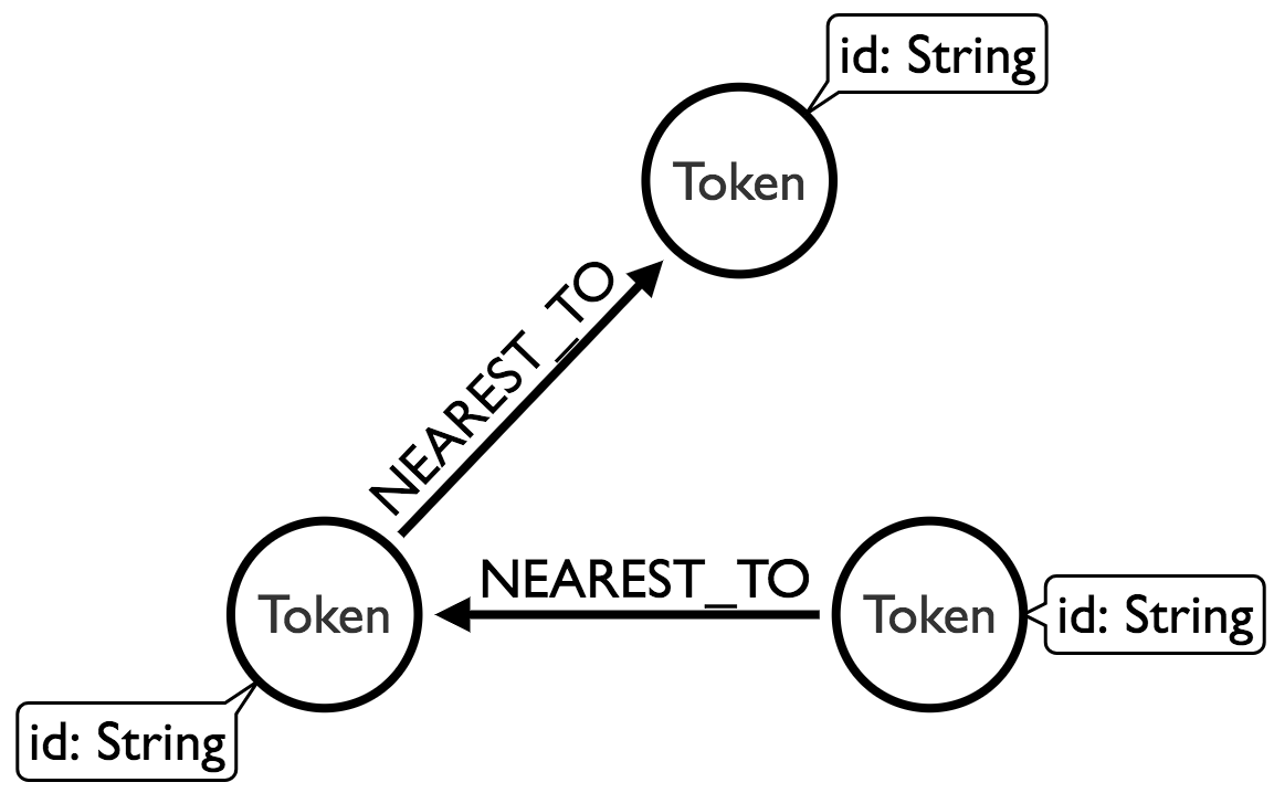
Each node will have an outgoing relationship to one other node, where the nearest neighbour is determine by comparing their embedding vectors with the euclidean distance function. This function does the trick:

def nearest_neighbour(label):
    with driver.session() as session:
        result = session.run("""\
        MATCH (t:`%s`)
        RETURN id(t) AS token, t.embedding AS embedding
        """ % label)

        points = {row["token"]: row["embedding"] for row in result}
        items = list(points.items())

        X = [item[1] for item in items]
        kdt = KDTree(X, leaf_size=10000, metric='euclidean')
        distances, indices = kdt.query(X, k=2, return_distance=True)

        params = []
        for index, item in enumerate(items):
            nearest_neighbour_index = indices[index][1]
            distance = distances[index][1]

            t1 = item[0]
            t2 = items[nearest_neighbour_index][0]
            params.append({"t1": t1, "t2": t2, "distance": distance})

        session.run("""\
        UNWIND {params} AS param
        MATCH (token) WHERE id(token) = param.t1
        MATCH (closest) WHERE id(closest) = param.t2
        MERGE (token)-[nearest:NEAREST_TO]->(closest)
        ON CREATE SET nearest.weight = param.distance
        """, {"params": params})

We would call the function like this:

nearest_neighbour("Token")

We can write a query to see what our graph looks like:

MATCH path = (:Token {id: "sons"})-[:NEAREST_TO]-(neighbour)
RETURN *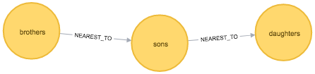

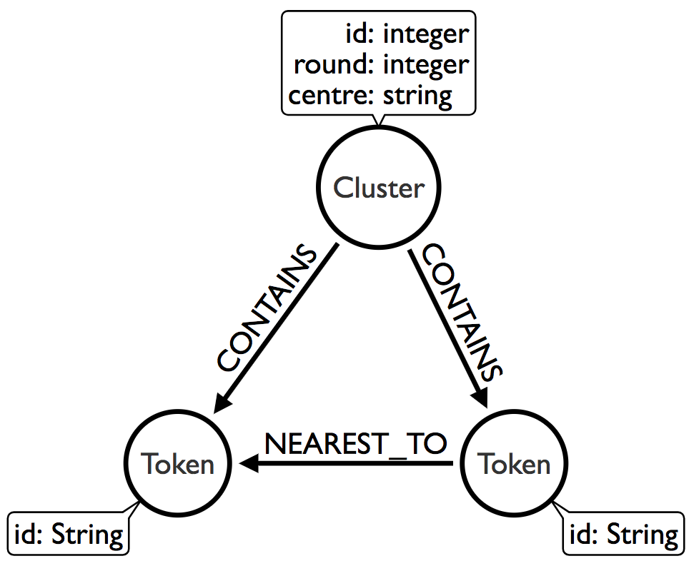
Connected components

After we’ve done that we need to run the connected components algorithm over the NNG. We’ll use the Union Find algorithm from the Neo4j Graph Algorithms library to help us out. This is the graph we want to have after this algorithm has run:

The following function finds the clusters:

def union_find(label, round=None):
    print("Round:", round, "label: ", label)
    with driver.session() as session:
        result = session.run("""\
            CALL algo.unionFind.stream(
              "MATCH (n:`%s`) RETURN id(n) AS id",
              "MATCH (a:`%s`)-[:NEAREST_TO]->(b:`%s`) RETURN id(a) AS source, id(b) AS target",
              {graph: 'cypher'}
            )
            YIELD nodeId, setId
            MATCH (token) WHERE id(token) = nodeId
            MERGE (cluster:Cluster {id: setId, round: {round} })
            MERGE (cluster)-[:CONTAINS]->(token)
            """ % (label, label, label), {"label": label, "round": round})

    print(result.summary().counters)

We would call the function like this:

round = 0
union_find("Token", round)

We can now write a function to find the cluster for our sons node and all of its sibling nodes:

MATCH path = (:Token {id: "sons"})<-[:CONTAINS]-()-[:CONTAINS]->(sibling)
RETURN *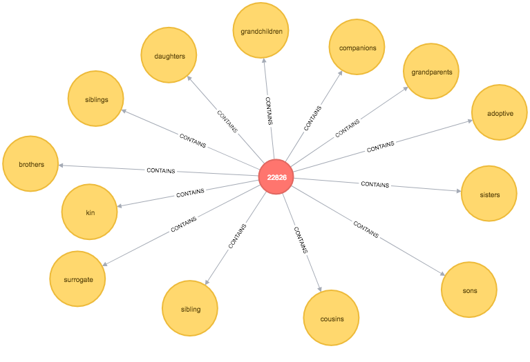

Now we need to make this process recursive.

Macro vertices

In the next part of the algorithm we need to find the central node for each of the clusters and then repeat the previous two steps using those nodes instead of all the nodes in the graph. We will consider the macro vertex node of each cluster to be the node that has the lowest cumulative distance to all other nodes in the cluster. The following function does this calculation:

def macro_vertex(macro_vertex_label, round=None):
    with driver.session() as session:
        result = session.run("""\
            MATCH (cluster:Cluster)
            WHERE cluster.round = {round}
            RETURN cluster
            """, {"round": round})

        for row in result:
            cluster_id = row["cluster"]["id"]

            session.run("""\
                MATCH (cluster:Cluster {id: {clusterId}, round: {round} })-[:CONTAINS]->(token)
                WITH cluster, collect(token) AS tokens
                UNWIND tokens AS t1 UNWIND tokens AS t2 WITH t1, t2, cluster WHERE t1 <> t2
                WITH t1, cluster, reduce(acc = 0, t2 in collect(t2) | acc + apoc.algo.euclideanDistance(t1.embedding, t2.embedding)) AS distance
                WITH t1, cluster, distance ORDER BY distance LIMIT 1
                SET cluster.centre = t1.id
                WITH t1
                CALL apoc.create.addLabels(t1, [{newLabel}]) YIELD node
                RETURN node
                """, {"clusterId": cluster_id, "round": round, "newLabel": macro_vertex_label})

This function also sets a centre property on each Cluster node so that we can more easily visualise the central node for a cluster. We would call it like this:

round = 0
macro_vertex("MacroVertex1", round)

Once this function has run we can write a query to find the similar words to sons at level 2:

MATCH path = (:Token {id: "sons"})<-[:CONTAINS]-()-[:CONTAINS]->(sibling)
OPTIONAL MATCH nextLevelPath = (sibling:MacroVertex0)<-[:CONTAINS]-()-[:CONTAINS]->(other)
RETURN *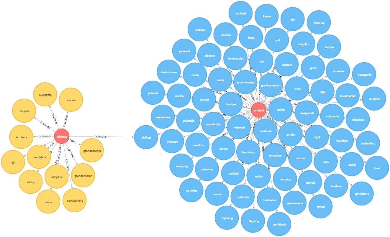

The output is quite cool - siblings is the representative node for our initial cluster and it takes us into a 2nd level cluster containing words such as uncles, sister-in-law, and nieces which do seem similar. There are some other words which are less so but I’ve only run this with a small sample of words so it’d be interesting to see how the algorithm fares if I load in a bigger dataset.

Next steps

I’ve run this over a set of 10,000 words, which took 23 seconds, and 50,000 words, which took almost 10 minutes. The slowest bit of the process is the construction of the Nearest Neighbour Graph. Thankfully this looks like a parallelisable problem so I’m hopeful that I can speed that up.

The code for this post is in the mneedham/interpreting-word2vec GitHub repository so feel free to experiment with me and let me know if it’s helpful or if there are ways that it could be more helpful.

About the author

I'm currently working on short form content at ClickHouse. I publish short 5 minute videos showing how to solve data problems on YouTube @LearnDataWithMark. I previously worked on graph analytics at Neo4j, where I also co-authored the O'Reilly Graph Algorithms Book with Amy Hodler.