
R: Bootstrap confidence intervals
I recently came across an interesting post on Julia Evans' blog showing how to generate a bigger set of data points by sampling the small set of data points that we actually have using bootstrapping. Julia’s examples are all in Python so I thought it’d be a fun exercise to translate them into R.
We’re doing the bootstrapping to simulate the number of no-shows for a flight so we can work out how many seats we can overbook the plane by.
We start out with a small sample of no-shows and work off the assumption that it’s ok to kick someone off a flight 5% of the time. Let’s work out how many people that’d be for our initial sample:
> data = c(0, 1, 3, 2, 8, 2, 3, 4)
> quantile(data, 0.05)
  5%
0.35
0.35 people! That’s not a particularly useful result so we’re going to resample the initial data set 10,000 times, taking the 5%ile each time and see if we come up with something better:
We’re going to use the sample function with replacement to generate our resamples:
> sample(data, replace = TRUE)
[1] 0 3 2 8 8 0 8 0
> sample(data, replace = TRUE)
[1] 2 2 4 3 4 4 2 2
Now let’s write a function to do that multiple times:
library(ggplot)

bootstrap_5th_percentile = function(data, n_bootstraps) {
  return(sapply(1:n_bootstraps,
                function(iteration) quantile(sample(data, replace = TRUE), 0.05)))
}

values = bootstrap_5th_percentile(data, 10000)

ggplot(aes(x = value), data = data.frame(value = values)) + geom_histogram(binwidth=0.25)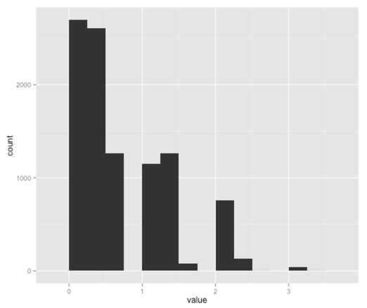
So this visualisation is telling us that we can oversell by 0-2 people but we don’t know an exact number.
Let’s try the same exercise but with a bigger initial data set of 1,000 values rather than just 8. First we’ll generate a distribution (with a mean of 5 and standard deviation of 2) and visualise it:
library(dplyr)

df = data.frame(value = rnorm(1000,5, 2))
df = df %>% filter(value >= 0) %>% mutate(value = as.integer(round(value)))
ggplot(aes(x = value), data = df) + geom_histogram(binwidth=1)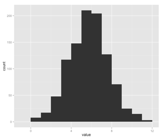
Our distribution seems to have a lot more values around 4 & 5 whereas the Python version has a flatter distribution - I’m not sure why that is so if you have any ideas let me know. In any case, let’s check the 5%ile for this data set:
> quantile(df$value, 0.05)
5%
 2
Cool! Now at least we have an integer value rather than the 0.35 we got earlier. Finally let’s do some bootstrapping over our new distribution and see what 5%ile we come up with:
resampled = bootstrap_5th_percentile(df$value, 10000)
byValue = data.frame(value = resampled) %>% count(value)

> byValue
Source: local data frame [3 x 2]

  value    n
1   1.0    3
2   1.7    2
3   2.0 9995

ggplot(aes(x = value, y = n), data = byValue) + geom_bar(stat = "identity")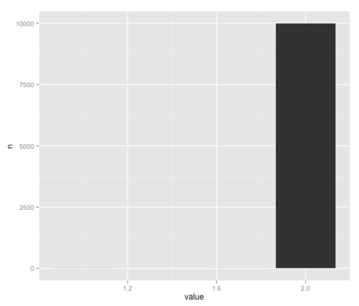
'2' is by far the most popular 5%ile here although it seems weighted more towards that value than with Julia’s Python version, which I imagine is because we seem to have sampled from a slightly different distribution.
About the author
I'm currently working on short form content at ClickHouse. I publish short 5 minute videos showing how to solve data problems on YouTube @LearnDataWithMark. I previously worked on graph analytics at Neo4j, where I also co-authored the O'Reilly Graph Algorithms Book with Amy Hodler.