9 Jul 2016

R: Sentiment analysis of morning pages

A couple of months ago I came across a cool blog post by Julia Silge where she runs a sentiment analysis algorithm over her tweet stream to see how her tweet sentiment has varied over time.

I wanted to give it a try but couldn’t figure out how to get a dump of my tweets so I decided to try it out on the text from my morning pages writing which I’ve been experimenting with for a few months.

Here’s an explanation of morning pages if you haven’t come across it before:

Morning Pages are three pages of longhand, stream of consciousness writing, done first thing in the morning. There is no wrong way to do Morning Pages — they are not high art. They are not even “writing.” They are about anything and everything that crosses your mind-- and they are for your eyes only. Morning Pages provoke, clarify, comfort, cajole, prioritize and synchronize the day at hand. Do not over-think Morning Pages: just put three pages of anything on the page…and then do three more pages tomorrow.

Most of my writing is complete gibberish but I thought it’d be fun to see how my mood changes over time and see if it identifies any peaks or troughs in sentiment that I could then look into further.

I’ve got one file per day so we’ll start by building a data frame containing the text, one row per day:

library(syuzhet)
library(lubridate)
library(ggplot2)
library(scales)
library(reshape2)
library(dplyr)

root="/path/to/files"
files = list.files(root)

df = data.frame(file = files, stringsAsFactors=FALSE)
df$fullPath = paste(root, df$file, sep = "/")
df$text = sapply(df$fullPath, get_text_as_string)

We end up with a data frame with 3 fields:

> names(df)

[1] "file"     "fullPath" "text"

Next we’ll run the sentiment analysis function - syuzhet#get_nrc_sentiment - over the data frame and get a score for each type of sentiment for each entry:

get_nrc_sentiment(df$text) %>% head()

  anger anticipation disgust fear joy sadness surprise trust negative positive
1     7           14       5    7   8       6        6    12       14       27
2    11           12       2   13   9      10        4    11       22       24
3     6           12       3    8   7       7        5    13       16       21
4     5           17       4    7  10       6        7    13       16       37
5     4           13       3    7   7       9        5    14       16       25
6     7           11       5    7   8       8        6    15       16       26

Now we’ll merge these columns into our original data frame:

df = cbind(df, get_nrc_sentiment(df$text))
df$date = ymd(sapply(df$file, function(file) unlist(strsplit(file, "[.]"))[1]))
df %>% select(-text, -fullPath, -file) %>% head()

  anger anticipation disgust fear joy sadness surprise trust negative positive       date
1     7           14       5    7   8       6        6    12       14       27 2016-01-02
2    11           12       2   13   9      10        4    11       22       24 2016-01-03
3     6           12       3    8   7       7        5    13       16       21 2016-01-04
4     5           17       4    7  10       6        7    13       16       37 2016-01-05
5     4           13       3    7   7       9        5    14       16       25 2016-01-06
6     7           11       5    7   8       8        6    15       16       26 2016-01-07

Finally we can build some 'sentiment over time' charts like Julia has in her post:

posnegtime <- df %>%
  group_by(date = cut(date, breaks="1 week")) %>%
  summarise(negative = mean(negative), positive = mean(positive)) %>%
  melt

names(posnegtime) <- c("date", "sentiment", "meanvalue")
posnegtime$sentiment = factor(posnegtime$sentiment,levels(posnegtime$sentiment)[c(2,1)])

ggplot(data = posnegtime, aes(x = as.Date(date), y = meanvalue, group = sentiment)) +
  geom_line(size = 2.5, alpha = 0.7, aes(color = sentiment)) +
  geom_point(size = 0.5) +
  ylim(0, NA) +
  scale_colour_manual(values = c("springgreen4", "firebrick3")) +
  theme(legend.title=element_blank(), axis.title.x = element_blank()) +
  scale_x_date(breaks = date_breaks("1 month"), labels = date_format("%b %Y")) +
  ylab("Average sentiment score") +
  ggtitle("Sentiment Over Time")

So overall it seems like my writing displays more positive sentiment than negative which is nice to know. The chart shows a rolling one week average and there isn’t a single week where there’s more negative sentiment than positive.

I thought it’d be fun to drill into the highest negative and positive days to see what was going on there:

> df %>% filter(negative == max(negative)) %>% select(date)

        date
1 2016-03-19

> df %>% filter(positive == max(positive)) %>% select(date)

        date
1 2016-01-05
2 2016-06-20

On the 19th March I was really frustrated because my boiler had broken down and I had to buy a new one - I’d completely forgotten how annoyed I was, so thanks sentiment analysis for reminding me!

I couldn’t find anything particularly positive on the 5th January or 20th June. The 5th January was the day after my birthday so perhaps I was happy about that but I couldn’t see any particular evidence that was the case.

Playing around with the get_nrc_sentiment function it does seem to identify positive sentiment when I wouldn’t say there is any. For example here’s some example sentences from my writing today:

> get_nrc_sentiment("There was one section that I didn't quite understand so will have another go at reading that.")

  anger anticipation disgust fear joy sadness surprise trust negative positive
1     0            0       0    0   0       0        0     0        0        1

> get_nrc_sentiment("Bit of a delay in starting my writing for the day...for some reason was feeling wheezy again.")

  anger anticipation disgust fear joy sadness surprise trust negative positive
1     2            1       2    2   1       2        1     1        2        2

I don’t think there’s any positive sentiment in either of those sentences but the function claims 3 bits of positive sentiment! It would be interesting to see if I fare any better with Stanford’s sentiment extraction tool which you can use with syuzhet but requires a bit of setup first.

I’ll give that a try next but in terms of getting an overview of my mood I thought I might get a better picture if I looked for the difference between positive and negative sentiment rather than absolute values.

The following code does the trick:

difftime <- df %>%
  group_by(date = cut(date, breaks="1 week")) %>%
  summarise(diff = mean(positive) - mean(negative))

ggplot(data = difftime, aes(x = as.Date(date), y = diff)) +
  geom_line(size = 2.5, alpha = 0.7) +
  geom_point(size = 0.5) +
  ylim(0, NA) +
  scale_colour_manual(values = c("springgreen4", "firebrick3")) +
  theme(legend.title=element_blank(), axis.title.x = element_blank()) +
  scale_x_date(breaks = date_breaks("1 month"), labels = date_format("%b %Y")) +
  ylab("Average sentiment difference score") +
  ggtitle("Sentiment Over Time")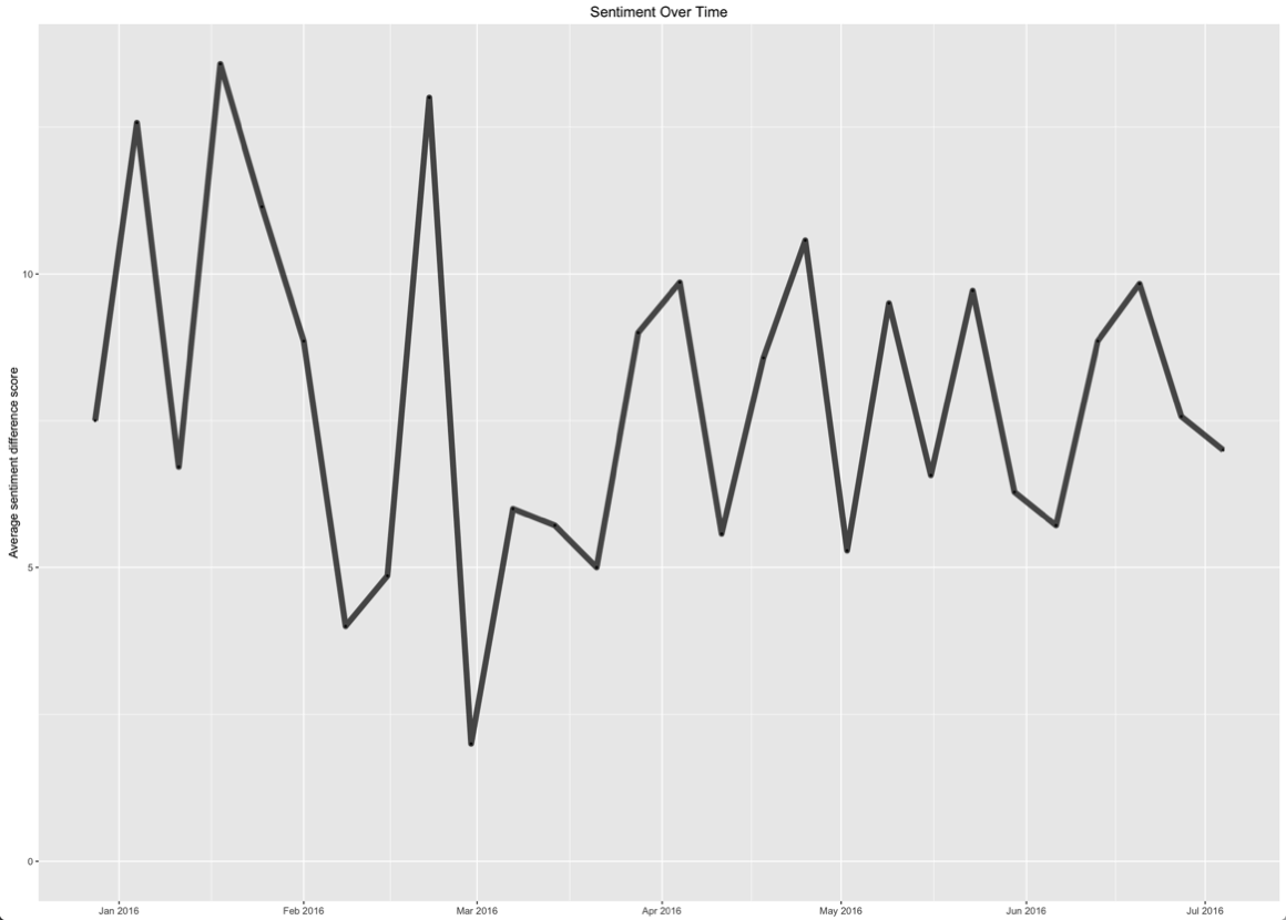

This one identifies peak happiness in mid January/February. We can find the peak day for this measure as well:

> df %>% mutate(diff = positive - negative) %>% filter(diff == max(diff)) %>% select(date)

        date
1 2016-02-25

Or if we want to see the individual scores:

> df %>% mutate(diff = positive - negative) %>% filter(diff == max(diff)) %>% select(-text, -file, -fullPath)

  anger anticipation disgust fear joy sadness surprise trust negative positive       date diff
1     0           11       2    3   7       1        6     6        3       31 2016-02-25   28

After reading through the entry for this day I’m wondering if the individual pieces of sentiment might be more interesting than the positive/negative score.

On the 25th February I was:

quite excited about reading a distributed systems book I’d just bought (I know?!)
thinking about how to apply the tag clustering technique to meetup topics
preparing my submission to PyData London and thinking about what was gonna go in it
thinking about the soak testing we were about to start doing on our project

</ul>

Each of those is a type of anticipation so it makes sense that this day scores highly. I looked through some other days which specifically rank highly for anticipation and couldn’t figure out what I was anticipating so even this is a bit hit and miss!

I have a few avenues to explore further but if you have any other ideas for what I can try next let me know in the comments.

About the author

I'm currently working on short form content at ClickHouse. I publish short 5 minute videos showing how to solve data problems on YouTube @LearnDataWithMark. I previously worked on graph analytics at Neo4j, where I also co-authored the O'Reilly Graph Algorithms Book with Amy Hodler.